Is Resident Advisor biased towards ambient music?

Jul 27, 2019

Joshua Feldman

8 minute read

Resident Advisor (or 'RA' for its loyal readership of DJs and crate diggers) is an online magazine dedicated to electronic music. Since its launch in 2001, RA has reviewed thousands of LPs/EPs, which have ranged in style from house and techno to dubstep and drum and bass.

After many years spent reading RA reviews, I started to suspect that the magazine has a bias towards ambient music - respective albums seemed to be receiving consistently good ratings and a disproportionate number of 'RA Recommends' awards.

Geek that I am, I decided to test this theory formally. Back in May, I scraped 15k+ reviews from the RA website using their parent URL, https://www.residentadvisor.net/reviews. I don't talk about the data cleaning in this blog post (you can see the data_preparation.R file on GitHub if you're really interested), but suffice it to say that I prepared a structured dataset with seven fields:

title: the name of the artist and the LP/EP
author: the name of the journalist who wrote the review
date: the date the review was published
genre: the genre(s) associated with the album
rating: a numerical score from 0.5 to 5.0
review: the original text of the review
ra_recommends: a binary indicator for whether the album received an 'RA Recommends' accolade

Using this information, I was able to test my two hypotheses:

Albums that are tagged as ambient have significantly higher ratings, on average.
Albums that are tagged as ambient are significantly more likely to be awarded 'RA Recommends'.

Preparation

Most of the data preparation occurred when I was ingesting the data in the first place. However, to aid the analysis, I will use one-hot encoding to add a series of dummy variables for the most common genres. For example, I'll add an ambient variable with two possible values: 1 if an album is tagged as ambient, and 0 if it is not.

library(tidyverse)
library(data.table)

df <- read_csv("https://github.com/joshua-feldman/resident-advisor/raw/master/resident-advisor.csv")

df <- df %>%
  mutate(ambient = as.factor(ifelse(genre == "ambient" | genre %like% "\\bambient\\b", 1, 0))) %>%
  mutate(deephouse = as.factor(ifelse(genre == "deephouse" | genre %like% "\\bdeephouse\\b", 1, 0))) %>%
  mutate(disco = as.factor(ifelse(genre == "disco" | genre %like% "\\bdisco\\b", 1, 0))) %>%
  mutate(dubstep = as.factor(ifelse(genre == "dubstep" | genre %like% "\\bdubstep\\b", 1, 0))) %>%
  mutate(electro = as.factor(ifelse(genre == "electro" | genre %like% "\\belectro\\b", 1, 0))) %>%
  mutate(experimental = as.factor(ifelse(genre == "experimental" | genre %like% "\\bexperimental\\b", 1, 0))) %>%
  mutate(house = as.factor(ifelse(genre == "house" | genre %like% "\\bhouse\\b", 1, 0))) %>%
  mutate(minimal = as.factor(ifelse(genre == "minimal" | genre %like% "\\bminimal\\b", 1, 0))) %>%
  mutate(techhouse = as.factor(ifelse(genre == "techhouse" | genre %like% "\\btechhouse\\b", 1, 0))) %>%
  mutate(techno = as.factor(ifelse(genre == "techno" | genre %like% "\\btechno\\b", 1, 0)))

Exploration

Now that the data is prepared, we are free to compare the distribution of ratings for ambient vs non-ambient music. We have a few options here - a boxplot or a violin plot would both be suitable - but I'll go with a density plot to show a smoothed version of each distribution along the x-axis.

df %>%
  filter(!is.na(ambient)) %>%
  ggplot(aes(rating, fill = ambient)) +
  geom_density(alpha = 0.5) +
  labs(title = "Density plot of Resident Advisor ratings for ambient vs non-ambient music",
       subtitle = "Based on 15k+ reviews from Feb 2001 to May 2019",
       x = NULL,
       y = NULL,
       caption = "Source: Resident Advisor") +
  guides(fill = FALSE) +
  geom_vline(xintercept = mean(df$rating[df$ambient==1], na.rm = TRUE),
             linetype = "dashed", col = "#00BFC4", size = 1) +
  geom_vline(xintercept = mean(df$rating[df$ambient==0], na.rm = TRUE),
             linetype = "dashed", col = "#F8766D", size = 1) +
  ggplot2::annotate("text", label = "Ambient", x = 4.5, y = 1,
                    family = "Raleway", col = "#00BFC4", fontface = "bold", size = 5) +
  ggplot2::annotate("text", label = "Not ambient", x = 4.5, y = 2,
                    family = "Raleway", col = "#F8766D", fontface = "bold", size = 5) +
  ggplot2::annotate("text", label = "The dashed lines represent the\nmean of each distribution",
                    x = 2.9, y = 2.35, family = "Raleway", size = 4)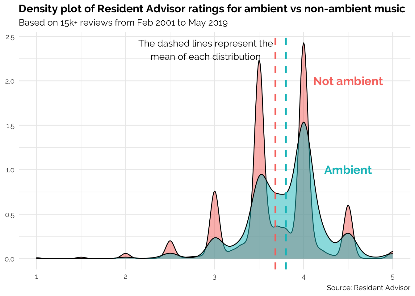

The density plot shows a clear difference in the distributions of ambient/non-ambient ratings. While the non-ambient distribution has well-defined peaks at .5 intervals (particularly at 3.5 and 4.0), the ambient distribution is flatter with a greater density of ratings between 3.5 and 4.0. Although the graph shows a difference between the mean of the two distributions, we don't yet know whether this difference is statistically significant.

Next, we will plot the percentage probability that each of the 10 most commonly reviewed genres - from ambient to techno - receives an 'RA Recommends' award.

df %>%
  select(ra_recommends, ambient:techno) %>%
  gather(genre, genre_flag, ambient:techno) %>%
  filter(genre_flag == 1) %>%
  group_by(genre) %>%
  summarise(ra_recommends = mean(as.numeric(ra_recommends), na.rm = TRUE)) %>%
  mutate(genre = reorder(genre, ra_recommends)) %>%
  mutate(label = paste(round(ra_recommends * 100, 2), "%", sep = "")) %>%
  mutate(ambient_flag = ifelse(genre == "ambient", 1, 0)) %>%
  ggplot(aes(genre, ra_recommends, label = label, fill = ambient_flag)) +
  geom_col() +
  geom_text(family = "Raleway", fontface = "bold", hjust = -0.1, size = 4) +
  geom_hline(yintercept = mean(df$ra_recommends), linetype = "dashed") +
  coord_flip() +
  labs(title = "Probability of 'RA Recommends' award for 10 most common genres",
       subtitle = "Based on 15k+ reviews from Feb 2001 to May 2019",
       x = NULL,
       y = NULL,
       caption = "Source: Resident Advisor") +
  scale_y_continuous(labels = scales::percent, limits = c(0, 0.06)) +
  guides(fill = FALSE) +
  ggplot2::annotate("text", x = 2, y = .0325, family = "Raleway", size = 4,
                    label = paste("Overall mean: ", round(mean(df$ra_recommends * 100), 2), "%", sep = ""))

## `summarise()` ungrouping output (override with `.groups` argument)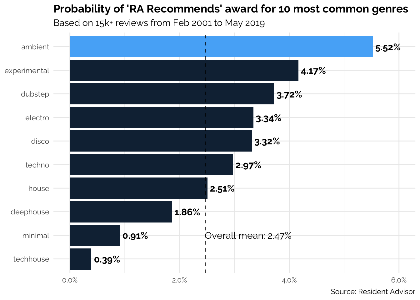

Here, the difference is a lot clearer: ambient albums have a greater chance of receiving an 'RA Recommends' award than any other major genre, with 5.52% of them receiving the accolade. It is worth noting that experimental - comparable to ambient in the abstraction of its musical form - is also more commended than average.

Analysis

Hypothesis #1

To test the first hypothesis, we will run a simple linear regression that predicts rating as a function of experimental. Since the Y variable is continuous and the X variable is binary categorical, this is equivalent to a two-sample t-test.

linear_model <- lm(rating ~ ambient, data = df)
summary(linear_model)

##
## Call:
## lm(formula = rating ~ ambient, data = df)
##
## Residuals:
##      Min       1Q   Median       3Q      Max
## -2.68236 -0.18236  0.01764  0.31764  1.31764
##
## Coefficients:
##             Estimate Std. Error t value Pr(>|t|)
## (Intercept) 3.682357   0.004182  880.59  < 2e-16 ***
## ambient1    0.117883   0.017780    6.63 3.47e-11 ***
## ---
## Signif. codes:  0 '***' 0.001 '**' 0.01 '*' 0.05 '.' 0.1 ' ' 1
##
## Residual standard error: 0.4988 on 15058 degrees of freedom
##   (635 observations deleted due to missingness)
## Multiple R-squared:  0.002911,   Adjusted R-squared:  0.002844
## F-statistic: 43.96 on 1 and 15058 DF,  p-value: 3.472e-11

The model shows that experimental albums are rated, on average, 0.12 points higher than non-experimental albums. This effect may be small, but it is significant at the 1% significance level, and we can therefore reject the null hypothesis that there is zero difference between the two groups.

Hypothesis #2

To test the second hypothesis, we will run a binary logistic regression that predicts ra_recommends as a function of experimental.

logistic_model <- glm(ra_recommends ~ ambient, data = df, family = "binomial")
summary(logistic_model)

##
## Call:
## glm(formula = ra_recommends ~ ambient, family = "binomial", data = df)
##
## Deviance Residuals:
##     Min       1Q   Median       3Q      Max
## -0.3371  -0.2180  -0.2180  -0.2180   2.7393
##
## Coefficients:
##             Estimate Std. Error z value Pr(>|z|)
## (Intercept) -3.72800    0.05537 -67.328  < 2e-16 ***
## ambient1     0.88841    0.16148   5.502 3.76e-08 ***
## ---
## Signif. codes:  0 '***' 0.001 '**' 0.01 '*' 0.05 '.' 0.1 ' ' 1
##
## (Dispersion parameter for binomial family taken to be 1)
##
##     Null deviance: 3546.8  on 15059  degrees of freedom
## Residual deviance: 3522.1  on 15058  degrees of freedom
##   (635 observations deleted due to missingness)
## AIC: 3526.1
##
## Number of Fisher Scoring iterations: 6

Since the model is logistic, its coefficients are given on the log odds scale. To work out the odds that an experimental album is recommended as opposed to a non-ambient album, we simply exponentiate the beta coefficient.

exp(logistic_model$coefficients[2])

## ambient1
## 2.431267

This suggests that an ambient album is 143% more likely to be recommended than a non-ambient album.

Conclusion

Lo and behold, RA does in fact have a bias towards ambient music - ambient albums are rated 0.12 points higher than non-ambient albums (p < 0.01) and are 143% more likely to be recommended (p < 0.01). Of course, this might be because of a genuine discrepancy in quality between the ambient and non-ambient music in RA's review catalogue; perhaps it reflects an 'objective' difference (insofar as there is objectivity in music perception), rather than a subjective bias on the part of the reviewers.

An alternative theory is that ambient music - at the abstract, often esoteric end of the electronic music spectrum - invokes a kind of social desirability bias, whereby the reviewer, forever wishing to flaunt their unorthodox taste, bends naturally towards the positive end of ambivalence. This way, if the reader doesn't enjoy the album being reviewed, they are the ones left feeling unsophisticated, apparently unable to appreciate the avant-garde.

In any case, the Resident Advisor dataset is now publicly available for your own explorations and musings. Enjoy!